nf-core/rnastructurome
a bioinformatics pipeline for analysing chemical high-throughput RNA structure-probing data
Introduction
This document describes the output produced by the pipeline. Most of the early steps (QC, trimming, alignment) follow standard RNA-seq conventions and their outputs are described in the nf-core/rnaseq documentation; this page focuses on the RNA Framework modules and downstream outputs specific to this pipeline.
Output layout
All paths are relative to the top-level output directory specified with --outdir.
<outdir>/├── fastqc/ (raw and post-trimming reads)├── cat/ (if multi-lane FASTQ merging occurs)├── cutadapt/├── star/├── bowtie/ (if --transcriptome)├── samtools/├── umi_tools/ (if UMI pattern provided)├── reference/│ ├── *.sorted.fa (Ensembl download only)│ ├── *.annotation.gtf.gz (Ensembl download only)│ ├── *.transcripts.fa (genome route, count_genome=false: transcript FASTA for browser viewing)│ ├── ensembl_fasta_source_url.txt│ └── ensembl_gtf_source_url.txt├── count/│ ├── rfcount_summary_all_samples.tsv│ └── <sample>/*.{rc,rci}├── norm/│ ├── <reference>.norm_factors.txt (if cross-experiment normalisation enabled)│ ├── <reference>.rfnormfactor.log│ ├── <group>_<replicate>/│ │ ├── xml/*.xml│ │ ├── wiggle/<group>.wig│ │ └── rfnorm.log│ ├── genome_bw/*.bw│ └── transcript_bw/*.bw├── correlate/ (if --correlate_replicates and >1 replicate)│ ├── <group>.{pearson,spearman}.rfcorrelate.log│ └── <group>.{pearson,spearman}_correlate/│ ├── matrix.csv│ └── pairwise/*.tsv├── fold/│ ├── <group>/│ │ ├── structures/r2dt/*.svg│ │ ├── structures/r2dt.log│ │ ├── structures/viennarna/*.svg│ │ ├── rdat/*.rdat│ │ ├── bp/*.bp│ │ ├── shannon/*.wig│ │ ├── rffold.log│ │ └── extracted_structures/ (if --structextract)│ │ ├── dotbracket/*.db (extracted motifs, dot-bracket)│ │ └── images/*_ss.svg (per-motif diagrams, reactivity-coloured)│ ├── genome_bp/*.bp│ ├── transcript_bp/*.bp│ ├── shannon_genome_bw/*.bw│ └── shannon_transcript_bw/*.bw├── jackknife/ (if --jackknife_reference provided)│ └── all_groups_jackknife/ (or <group>_jackknife/ per group if --rfjackknife_pool_all false)│ ├── mFMI.csv│ └── rfjackknife.log├── eval/ (if --rfeval_reference provided)│ └── <group>/│ ├── <group>_rfeval.metrics.tsv│ ├── rfeval.log│ └── plots/ (if --rfeval_img)├── multiqc/└── pipeline_info/Standard steps (QC, trimming, alignment)
Read QC (FastQC), adapter trimming (Cutadapt), alignment (STAR), and SAMtools post-processing follow standard nf-core/rnaseq conventions. See the nf-core/rnaseq output documentation for a description of those output files.
FastQC is run twice per sample and both reports are published to fastqc/: once on the raw input reads (<sample>_{1,2}_fastqc.*) and once on the Cutadapt-trimmed reads (<sample>_trimmed_trimmed_{1,2}_fastqc.*), so you can compare read quality before and after trimming.
Reference files
Output files
reference/ensembl_fasta_source_url.txt: URL of the FASTA file downloaded from Ensembl, for provenance.ensembl_gtf_source_url.txt: URL of the GTF file downloaded from Ensembl, for provenance.<organism>.sorted.fa: Chromosome-sorted reference FASTA, ready for reuse in subsequent runs via--fasta.<organism>.annotation.gtf.gz: Ensembl gene annotation GTF, ready for reuse via--gtf.<reference>.transcripts.fa: Genome route with the defaultcount_genome = falseonly. Transcript sequences extracted from the genome FASTA and GTF (viagffread), matching the transcript IDs used in the count/norm/fold outputs. Load this as the reference in a genome browser to view the transcript-coordinate tracks (see below).
The source-URL and sorted.fa / annotation.gtf.gz files are published only when the reference is downloaded automatically from Ensembl (i.e. --fasta was not provided); when a local FASTA is supplied, those are not re-published. The sorted FASTA can be passed directly to subsequent runs to skip the download step. The transcripts.fa file is published whenever the genome route runs (regardless of reference source), because the genome route otherwise has no single transcript FASTA to view the transcript-coordinate tracks against.
RNA Framework
This pipeline uses modules from RNA Framework.
rf-count
Output files: transcriptome route
count/rfcount_summary_all_samples.tsv: Aggregatedrf-countsummary across all samples in the run (the per-sample summaries are merged into this single TSV for easy comparison between samples).count/<sample>/<sample>.rc: Transcript-level raw per-position count file used as input torf-norm.index.rci: Index sidecar for the transcript-level count file.
Output files: genome route
count/<sample>/<sample>.plus.rc/<sample>.minus.rc: Genome-coordinate strand-specific raw count files.<sample>.rc: Transcript-level count file extracted from genome coordinates viarf-rctools extract, used as input torf-norm.<sample>.rc.rci: Index sidecar for the transcript-level count file.- The aggregated
count/rfcount_summary_all_samples.tsv(above) also covers genome-route samples.
rf-count calculates per-base RT-stop or mutation counts and read coverage from aligned reads. In most cases, the pipeline runs rf-count directly against transcript-coordinate BAM files provided by STAR or Bowtie. Optionally, it runs rf-count-genome on the genome aligned BAM first, then converts genome-coordinate count files to transcript-level .rc files with rf-rctools extract.
The transcript-level <sample>.rc and <sample>.rc.rci files are passed to rf-norm for reactivity normalisation.
Example rfcount_summary_all_samples.tsv
The aggregated summary reports, per sample, the number of transcripts covered and the per-base composition of the counted events (pct_a_muts…pct_u_muts). The exact column set depends on the counting mode: MaP counts mismatches within each alignment, so it can report the overall mutated-alignment fraction (mutated_alignments, pct_mutated); RT-stop counts reverse-transcriptase drop-off positions rather than per-read mutations, so those two columns do not apply and are omitted. As a sanity check on the chemistry, in MaP runs pct_mutated should be higher in the treated samples than in the untreated controls. For DMS specifically (at pH < 8, where it modifies mainly A and C), pct_a_muts and pct_c_muts should dominate over pct_g_muts and pct_u_muts.
MaP (mutational profiling) (SHAPE)
| sample | covered | mutated_alignments | pct_mutated | pct_a_muts | pct_c_muts | pct_g_muts | pct_u_muts |
|---|---|---|---|---|---|---|---|
| MDA-MB-231_DMSO_treated_r1 | 20241 | 106400534/151175161 | 70.38 | 19.59 | 21.41 | 26.94 | 32.06 |
| MDA-MB-231_DMSO_treated_r2 | 20508 | 109647170/159460915 | 68.76 | 19.83 | 20.65 | 27.11 | 32.42 |
| MDA-MB-231_DMSO_untreated_r1 | 24171 | 294831112/1121966212 | 26.28 | 20.30 | 29.69 | 28.89 | 21.11 |
| MDA-MB-231_DMSO_untreated_r2 | 24482 | 351733856/1409123432 | 24.96 | 20.84 | 25.96 | 30.87 | 22.33 |
| MDA-MB-231_MTX_treated_r1 | 20639 | 121944486/180812092 | 67.44 | 20.05 | 21.29 | 25.81 | 32.84 |
| MDA-MB-231_MTX_treated_r2 | 20473 | 108016250/155999073 | 69.24 | 20.27 | 20.68 | 26.33 | 32.71 |
This is close to an ideal result: the treated samples sit at ~67-70% pct_mutated against ~25% in the untreated controls, a clean ~3× separation that shows the probe reacted well above background.
RT-stop (DMS)
| sample | covered | pct_a_muts | pct_c_muts | pct_g_muts | pct_u_muts |
|---|---|---|---|---|---|
| L26_Delta_Rep1_100mM_DMS_r1 | 4278 | 48.48 | 12.43 | 17.03 | 22.06 |
| L26_Delta_Rep1_100mM_DMS_r2 | 4734 | 39.09 | 15.35 | 21.21 | 24.36 |
| L26_Delta_Rep1_NoDMS_r1 | 4369 | 32.74 | 15.94 | 20.74 | 30.58 |
| L26_Delta_Rep1_NoDMS_r2 | 5016 | 26.71 | 18.95 | 24.30 | 30.03 |
| Scer_WT_NoDMS_r1 | 4117 | 31.88 | 16.59 | 21.51 | 30.02 |
| Scer_WT_NoDMS_r2 | 5038 | 26.31 | 18.98 | 24.63 | 30.07 |
| WT_Rep1_100mM_DMS_r1 | 4223 | 47.23 | 12.81 | 18.34 | 21.62 |
| WT_Rep1_100mM_DMS_r2 | 4584 | 39.38 | 15.08 | 20.99 | 24.56 |
This example is less clear-cut. Lacking pct_mutated (see above), the base composition is the main handle: pct_a_muts does rise in the DMS-treated samples (~39-48% vs ~26-32% in the controls), but pct_c_muts is not elevated as DMS at pH < 8 would predict. Results like this warrant a closer look at the downstream reactivities before drawing conclusions.
rf-normfactor (optional)
Output files
norm/<reference>.norm_factors.txt: Transcriptome-wide, cross-experiment normalisation factors for the reference, applied to every group’srf-normvia-nf.norm/<reference>.rfnormfactor.log: Rawrf-normfactorconsole output.
rf-normfactor derives a single set of normalisation factors across all samples in a dataset aligned to the same reference so that reactivities are on a common scale for cross-sample comparison. This is auto-enabled for a reference with more than one treated sample. When it does not run, rf-norm normalises each group independently and no factor file is produced.
Example <reference>.rfnormfactor.log
The log records how many bases were covered across all of the reference’s samples, how many of those were selected for normalisation, and the resulting per-sample factor that is passed to each treated group’s rf-norm via -nf. Only treated samples receive a factor; untreated controls contribute to scoring but are not listed here.
[+] Loading RC files...[+] Calculating raw reactivities for bases covered across all samples... 810287 bases selected.[+] Freeing unused memory...[+] Selecting bases for normalization... 10700 selected.[+] Normalization factors:
  [*] MDA-MB-231_DMSO_treated_r1: 0.0303267245741193  [*] MDA-MB-231_DMSO_treated_r2: 0.0307702477985242  [*] MDA-MB-231_MTX_treated_r1: 0.0274075148970783  [*] MDA-MB-231_MTX_treated_r2: 0.0315441960095623
[+] All done.
The factors within a reference should be broadly comparable across samples; a sample with a wildly different factor is worth investigating.
rf-norm
Output files
norm/<group>/xml/<transcript>.xml: Normalised reactivity profiles in RNA Framework XML format, used as input forrf-foldand optionallyrf-jackknife.rfnorm.log: Rawrf-normconsole output.wiggle/<group>.wig: Reactivity wiggle track for the group, produced byrf-wiggleover all of the group’s normalised transcript XMLs. This is a single WIG file with one section per transcript (not one file per transcript).
norm/genome_bw/<sample_group>_reactivity_genome.bw: Genomic-coordinate reactivity BigWig. When multiple replicates are present the per-replicate transcript-level tracks are averaged position-by-position, remapped to genomic coordinates using the GTF, and converted to BigWig format.
norm/transcript_bw/<sample_group>_reactivity_transcript.bw: Transcript-coordinate reactivity BigWig. Same averaged reactivity data asgenome_bw/but in transcript coordinates, suitable for visualisation alongside transcript-level annotations.
rf-norm normalises raw RT-stop or MaP counts into per-nucleotide reactivity scores. Reactivity reflects each nucleotide’s accessibility to the probe: high reactivity indicates an unpaired, flexible base, while low reactivity indicates a paired or structurally protected one. Output is grouped by sample_group + replicate (e.g. HEK293T_1). The XML files are the primary output passed to downstream structure-prediction steps. The BigWigs provide reactivity tracks (averaged across replicates where applicable) in both genomic and transcript coordinates for genome browser visualisation.
Example rfnorm.log
This log summarises how many transcripts were normalised and why others were dropped:
[+] Normalization statistics:
  [*] Covered transcripts:   2264  [*] Discarded transcripts: 30203 total                             30203 insufficient coverage                             0 mismatch between treated and untreated sample sequence                             0 absent in untreated sample reference
[+] All done.
Most transcripts are typically discarded for insufficient coverage; the mismatch and absent-in-untreated counts should stay at or near zero, as non-zero values there point to a reference or sample-pairing problem rather than shallow coverage.
The reactivity BigWigs (norm/{genome,transcript}_bw/) can be loaded into a genome browser such as IGV; see Viewing tracks in a genome browser for which reference to load per route, example figures, and interpretation caveats.
rf-correlate (replicate QC)
Output files
correlate/<group>.pearson_correlate/andcorrelate/<group>.spearman_correlate/matrix.csv: Overall pairwise correlation matrix between the group’s replicates.pairwise/<repA>_vs_<repB>.tsv: Per-transcript correlation coefficients and p-values for each replicate pair.
correlate/<group>.{pearson,spearman}.rfcorrelate.log: Rawrf-correlateconsole output for each method.
rf-correlate quantifies replicate reproducibility by correlating reactivity profiles between the replicates of a sample group (transcriptome-wide and per-transcript). It runs for groups with more than one replicate (controlled by --correlate_replicates) and computes both Pearson (reactivity-capped) and Spearman (rank-based) correlations, published to separate .pearson/.spearman directories. The overall pairwise correlations are also summarised in the MultiQC report as a per-sample-group table (number of replicates, mean Pearson and mean Spearman correlation), giving an at-a-glance reproducibility check.
Example rfcorrelate.log
Each log reports how many transcripts were shared across the group’s replicates, the pairwise correlation, and how many transcripts had enough paired positions to be correlated:
[+] Importing input XML directories/files... 2144 common transcripts.[+] Calculating pairwise correlations...
[+] Pairwise correlations (over 855878 bases):
  Sample #1    Sample #2    Correlation    p-value
  rep1_1       rep2_2       0.765          0.00e+00
[+] Correlation statistics:
  [*] Correlated transcripts/blocks: 2141  [*] Discarded transcripts/blocks:  3 total                                     0 parsing failed                                     0 mismatch between transcript sequences                                     3 not enough values for correlation calculation
[+] All done.
The headline number is the pairwise correlation (here Pearson 0.765 between the two DMSO replicates); higher means more reproducible reactivity profiles, and it is the value carried into the MultiQC table. Discards are almost always transcripts with too few paired positions to correlate; non-zero parsing failed or mismatch between transcript sequences counts instead indicate a reference or input problem.
rf-fold
Output files
fold/<group>/structures/r2dt/<transcript>.svg: Template-based 2D structure diagram drawn by R2DT, when a matching template is available.structures/viennarna/<transcript>.svg: RNAplot 2D structure diagram drawn by ViennaRNA.structures/r2dt.log: log of transcripts drawn/skipped by R2DT.rdat/<transcript>.rdat: RDAT-format file (compatible with RMDB) which summarises results (sequence, dot-bracket notation, reactivities) and key parameters for how it was produced.bp/<transcript>.bp: Per-transcript base-pair arcs in transcript coordinates, keeping pairs at 10% probability or above. These are merged into the transcript-coordinate.bpfile below.shannon/<transcript>.wig: Per-transcript Shannon entropy in transcript coordinates. These are merged into the genome or transcript-coordinate BigWigs below.rffold.log: Rawrf-foldconsole output.
fold/genome_bp/<sample_group>_genome.bp: Base-pair arcs merged into a single file per sample group in genome coordinates, suitable for arc diagram visualisation in a genome browser such as IGV.
fold/transcript_bp/<sample_group>_transcript.bp: Same base-pair arcs in transcript coordinates (transcript ID as chromosome, 1-based transcript positions). Suitable for visualisation against a transcript-level reference in IGV.
fold/shannon_genome_bw/<sample_group>_shannon_genome.bw: Genomic-coordinate per-position Shannon entropy BigWig across the transcript ensemble for a sample group.
fold/shannon_transcript_bw/<sample_group>_shannon_transcript.bw: Transcript-coordinate Shannon entropy BigWig, equivalent toshannon_genome_bw/but in transcript coordinates.
rf-fold predicts RNA secondary structures from normalised reactivity profiles. Replicates for the same sample group are combined and folded together using ViennaRNA RNAfold in a windowed manner, which improves accuracy for long transcripts by folding overlapping sequence windows and merging the results. Key outputs per transcript include 2D structure diagrams, RDAT files summarising the predicted structure and reactivity values. Genome-wide Shannon entropy profiles and base-pair arcs are additionally provided as BigWig and .bp tracks for visualisation in a genome browser, in both genome and transcript coordinates. Shannon entropy measures the uncertainty of the predicted base-pairing at each position: lower entropy means the structure ensemble agrees on a single conformation (a higher-confidence prediction), while higher entropy indicates several competing folds.
The two renderers run independently in parallel, so a transcript with an R2DT template gets both diagrams:
- ViennaRNA: draws every transcript.
RNAplotproduces an energy-minimised 2D diagram from the dot-bracket structure. Published tofold/<group>/structures/viennarna/. - R2DT: additionally draws transcripts with a matching template in the R2DT library (rRNA, snRNA, tRNA, etc.), producing layouts comparable across organisms. Enabled with
--r2dt. Published tofold/<group>/structures/r2dt/.
Example structure diagram
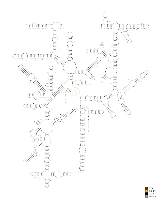
R2DT lays the predicted structure onto a standard template so diagrams are comparable across samples and organisms. The example below is the E. coli 16S rRNA (fold/E_coli_DH5a_ex_vivo/structures/r2dt/16S.svg), matched to the R2DT small-subunit rRNA template:
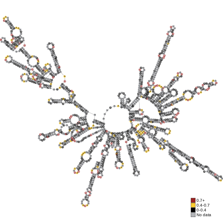
ViennaRNA RNAplot draws the same predicted structure with an energy-minimised layout rather than a standard template. Because both renderers run, a transcript like 16S is drawn both ways: here is the same E. coli 16S rRNA drawn by ViennaRNA (fold/E_coli_DH5a_ex_vivo/structures/viennarna/16S.svg):
Example .rdat file
The per-transcript RDAT file bundles the sequence, the predicted structure, and the reactivity data behind these diagrams into one RMDB-compatible record. Below is the E. coli 16S rRNA RDAT with the long sequence/structure/reactivity lines abbreviated:
NAME 16S rRNASEQUENCE AAAUUGAAGAGUUUGAUCAUGGCUCAGAUUGAACGCUGGCGGCAGGCCUAACACAUGCAAGUCGAACGGUAACAGGAAGAAGCUUGCUUCUUUGCUGACG…STRUCTURE ........(((((.......)))))......((((((.(((((((((((..(((.(((..(((....(((((..(((((.......))))))))))))).…ANNOTATION_DATA:1 modifier:DMSREACTIVITY 0 0 0 NaN NaN NaN 0.053 0.065 NaN 0.012 NaN NaN NaN NaN NaN 0.024 NaN 0.05 0.252 NaN NaN NaN 0.01 NaN 0.089 0.482 NaN 0.057 NaN NaN NaN 0.044 0.041 0.019 NaN 0.022 NaN NaN NaN 0.021 NaN NaN 0.023 0.235 NaN NaN 0.024 0.078 NaN 0.562 0.869 0.154 0.122 0.108 0.352 NaN NaN 0.055 0.857 0.44 NaN NaN 0.037 NaN 0.927 0.759 2.555 NaN NaN NaN 0.2 0.224 0.026 0.064 NaN NaN 0.021 0.036 NaN 2.938 0.034 NaN 0.073 NaN NaN NaN 0.008 NaN NaN 0.022 NaN NaN NaN NaN 0.045 NaN NaN 0.115 0.068 …COMMENT Generated by nf-core/rnastructurome v1.0.0dev; FASTA: ecoli_rrna_collab.fa; Principle: MaP; rf-norm scoring: sm=4 (Zubradt); normalisation: nm=3 (Box-plot)The fields are: NAME (transcript ID), SEQUENCE, STRUCTURE (predicted structure in dot-bracket notation), ANNOTATION_DATA (the probe used, here DMS), REACTIVITY (per-nucleotide normalised reactivity, NaN where there was no usable signal), and COMMENT (provenance: pipeline version, reference FASTA, probing principle, and the rf-norm scoring/normalisation methods used to produce the values).
Viewing tracks in a genome browser
The reactivity and Shannon-entropy BigWigs (norm/{genome,transcript}_bw/, fold/shannon_{genome,transcript}_bw/) load into IGV or UCSC against the matching reference:
- Genome-coordinate tracks (
*_genome.bw,fold/genome_bp/): load against the genome FASTA + GTF. On the transcriptome route these are not produced; use the genome route if you want a genomic view. - Transcript-coordinate tracks (
*_transcript.bw,fold/transcript_bp/): load the transcript FASTA as the browser’s reference sequence: the transcriptome route’s<organism>.sorted.fa(the cDNA FASTA), orreference/<reference>.transcripts.faon the default (count_genome = false) genome route. Each transcript appears as its own “chromosome”, so the per-nucleotide profile is continuous.
Genome tracks superpose isoforms; prefer transcript coordinates for structure
Genome-coordinate tracks project every transcript onto the assembly and average overlapping positions, so at a multi-isoform locus (e.g. human HLA-A and the rest of the MHC) the track is a superposition of all isoforms, not the profile of any single transcript. This matters differently for the two kinds of data:
- Reactivity is a per-nucleotide experimental measurement, so its genome projection is meaningful: it shows where the RNA was modified, and gaps mark introns or uncovered positions. It only writes covered positions, so introns of a given transcript stay empty unless another isoform genuinely has a covered exon there.
- Shannon entropy and base-pair arcs describe the fold of a whole transcript, not a genomic position, and are defined at every folded nucleotide (no coverage gaps). Projected to the genome and averaged across isoforms, they blend distinct structural models: one isoform’s introns get filled by another isoform’s exons, so the track looks continuous across the locus. This is expected, not a bug, but it is not “the structure” of any one transcript.
For accurate interpretation, prefer the transcript-coordinate tracks against the transcript FASTA, where each transcript is its own “chromosome” with no cross-isoform blending. The genome-coordinate tracks are best used to visualise reactivity profiles in the context of the surrounding transcripts/locus, rather than as a per-transcript structural readout. On single-isoform genes (and all prokaryotic references, which are unspliced) the genome and transcript views are equivalent and this caveat does not apply.
Example figures
All figures below are from the human HLA-A gene (SHAPE, MDA-MB-231).
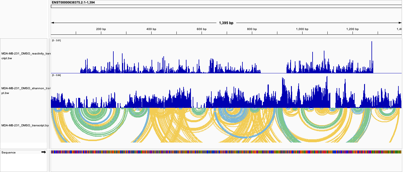
All tracks together (transcript coordinates). Reactivity, Shannon entropy, and base-pair arcs for a single transcript (ENST00000638375, DMSO), loaded against the transcript FASTA. This is the cleanest way to read a single transcript’s data: every track shares the same continuous per-nucleotide axis:
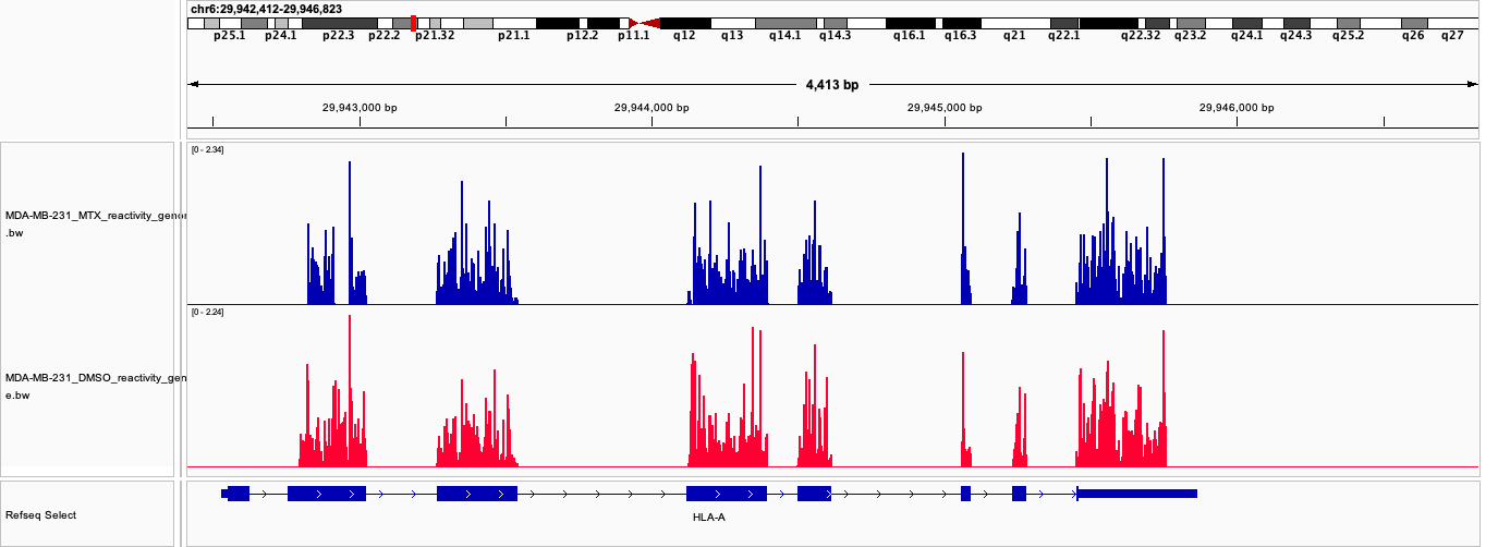
Reactivity in genome coordinates (norm/genome_bw/<group>_reactivity_genome.bw). Signal follows the exon structure of the gene model, with introns appearing as gaps; the genome view is meaningful for reactivity because it is a per-nucleotide measurement:
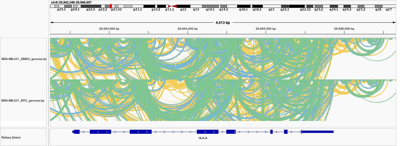
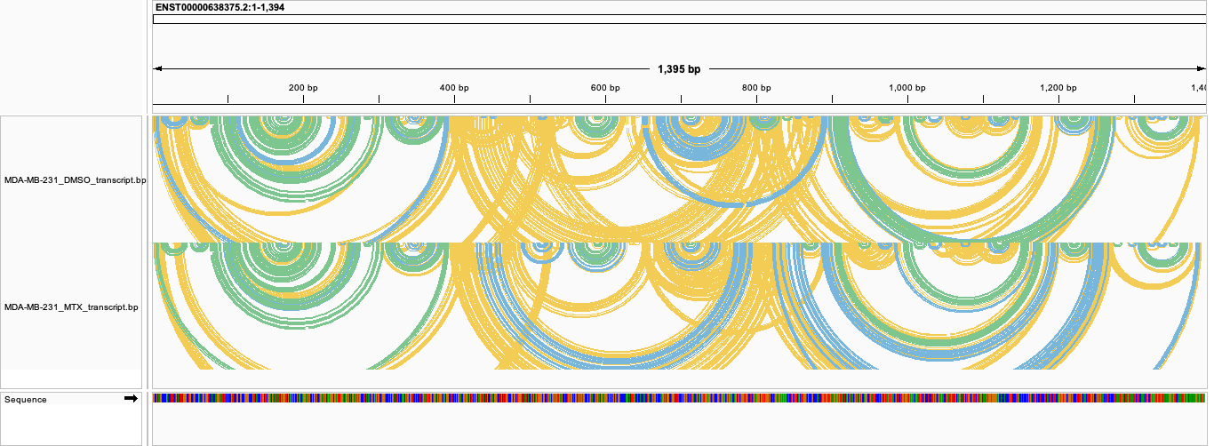
For structure, the genome view is less useful at a multi-isoform locus like HLA-A. In the base-pair arc tracks, each arc connects two paired bases, coloured by base-pair probability: yellow = 10-40%, blue = 40-70%, green = 70-100% (pairs below 10% are not drawn; rf-fold’s dot-plot conversion runs with --min-color-index 1).
Genome-coordinate base-pair arcs (fold/genome_bp/<group>_genome.bp): base pairs from every folded isoform are projected onto the assembly and overlap into a dense tangle:
Transcript-coordinate base-pair arcs (fold/transcript_bp/<group>_transcript.bp): the same data for one transcript, showing clean nested arcs:
The Shannon-entropy tracks (fold/shannon_{genome,transcript}_bw/) behave the same way: clean per transcript, superposed in genome coordinates.
rf-structextract (optional)
Output files
fold/<group>/extracted_structures/dotbracket/*.db: Extracted structural motifs for the sample group in dot-bracket notation (one multi-record file per transcript, each record named<transcript>_<start>-<end>), filtered to high-confidence, low-reactivity / low-Shannon elements meeting the configured criteria.fold/<group>/extracted_structures/images/*_ss.svg: One 2D diagram per extracted motif, drawn with ViennaRNA RNAplot and coloured by SHAPE reactivity in the same style as the rf-fold structure plots.
rf-structextract extracts well-defined structural elements from the rf-fold output by combining the predicted structures with per-base reactivity and Shannon entropy. Only runs when --structextract is set (see usage docs for the selection-criteria parameters). It identifies substructures whose bases are consistently below the transcript median for both reactivity and Shannon entropy, which is the signature of stably folded regions.
Example extracted motif
This is where rf-structextract earns its place: it pulls the few genuinely well-defined structural elements out of a large transcript, where the full-length fold is mostly low-confidence and hard to read. The human transcript ENST00000942651 (2,173 nt, MDA-MB-231_DMSO group) is a good example: its full rf-fold ViennaRNA diagram (fold/MDA-MB-231_DMSO/structures/viennarna/ENST00000942651.svg) is a dense, largely uninformative hairball:
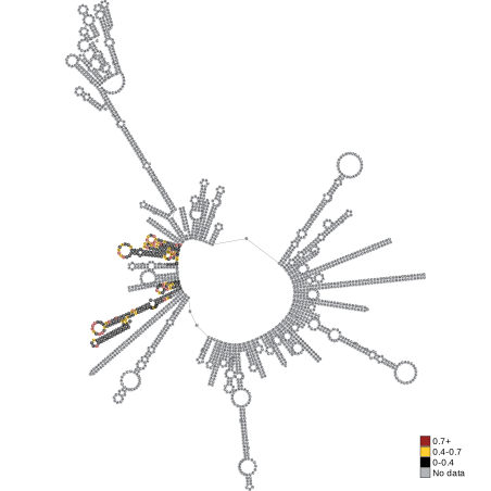
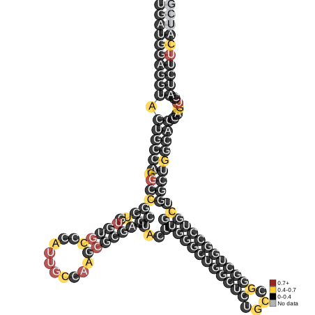
From this, rf-structextract isolates one region, positions 646-750, whose bases pass the reactivity and Shannon-entropy tests, a well-defined 105 nt motif that would otherwise be lost in the full-length diagram. It is written to the multi-record dot-bracket file (extracted_structures/dotbracket/ENST00000942651.db, record ENST00000942651_646-750) and drawn on its own, reactivity-coloured, in extracted_structures/images/ENST00000942651_646-750_ss.svg:
rf-jackknife (optional)
Output files
jackknife/all_groups_jackknife/(the default pooled run; with--rfjackknife_pool_all falseyou instead get onejackknife/<group>_jackknife/per sample group)mFMI.csv: Grid-search scores as a semicolon-delimited matrix. Rows are slope values, columns are intercept values, and each cell is the mean modified Fowlkes-Mallows Index (mFMI) between the reference structures and the structure rf-fold predicts at that slope/intercept.rfjackknife.log: Rawrf-jackknifeconsole output, including the ranked top slope/intercept pairs and the jackknifing statistics.
rf-jackknife identifies optimal slope and intercept parameters for reactivity-guided structure folding by performing a grid search and comparing predicted structures to a set of reference structures using the (modified) Fowlkes-Mallows Index.
This step only runs when --jackknife_reference is provided.
Example mFMI.csv and log
Below is a bacterial calibration (jackknife/all_groups_jackknife/, DMS-MaP scored against two reference structures, 16S and 23S rRNA). Rows are slopes, columns are intercepts, and higher mFMI is better; the scores climb towards the high-slope, low-magnitude-intercept corner (columns abbreviated):
mFMI;-3;-2.8;…;-1.6;-1.4;…;-0.20;0.483;0.484;…;0.567;0.573;…;0.6542.2;0.691;0.734;…;0.810;0.820;…;0.8404.4;0.817;0.819;…;0.859;0.867;…;0.8264.8;0.818;0.831;…;0.867;0.859;…;0.829rf-jackknife ranks the best pairs and reports how many transcripts contributed in the log:
[+] Top slope/intercept value pairs:
  Slope    Intercept    mFMI
  4.4      -1.4         0.867  4.8      -1.6         0.867  4.6      -1.4         0.866  4.6      -1.6         0.864  3.4      -1.2         0.860
[+] Jackknifing statistics:
  [*] Used transcripts:     2  [*] Excluded transcripts: 0 total
Here the optimal pair is slope 4.4 / intercept -1.4 (mFMI 0.867). mFMI runs from 0 to 1, where around 0.5 is no better than chance and higher means closer agreement with the reference structures; as a rough guide a best value above 0.7 indicates a genuinely well-calibrated fold, so 0.867 here is a strong result. When jackknife runs, these calibrated values take priority over the --rffold_slope/--rffold_intercept flags and the chemical-based defaults, and are passed on to rf-fold (unless --stop_after_jackknife is set).
rf-eval (optional)
Output files
eval/<group>/<group>_rfeval.metrics.tsv: Per-structure agreement metrics, each paired with its rotation baseline. The main result of the step.rfeval.log: Rawrf-evalconsole output, in two labelled blocks: the reference structures, then the rotation baseline (which reports a much larger structure count, since it scores every decoy).plots/(only with--rfeval_img): per-structure DSCI plots underplots/dsci/, plusroc.pdfandsummary.pdf.
rf-eval evaluates how well normalised reactivity profiles agree with a set of reference structures. It reports three metrics, each running from 0 to 1:
- Unpaired Coefficient: fraction of highly reactive bases that are unpaired
- DSCI: probability that a randomly selected unpaired base has higher reactivity than a paired base
- AUROC: area under the ROC curve treating reactivity as a classifier of unpaired bases
Each metric is written next to its own rotation baseline (see usage docs) as <metric>_baseline_mean and <metric>_baseline_sd, with baseline_num giving the decoy count behind them (the structure’s length minus 9, since rotations are enumerated and near-identity shifts skipped).
This step only runs when --rfeval_reference is provided.
Example metrics
Zika virus MR766 in vivo, scored against six Rfam reference elements with --rfeval_windows (baseline columns abridged to mean/sd):
structure coeff_unpaired mean sd dsci mean sd auroc mean sd baseline_numzika_5UTR 0.8750 0.5479 0.0930 0.6006 0.3782 0.0568 0.7127 0.4969 0.0595 152zika_CRE_3UTR 0.8333 0.5398 0.0797 0.4085 0.2733 0.0385 0.6495 0.4947 0.0418 89zika_DB_3UTR 0.8750 0.4923 0.0615 0.8074 0.4128 0.0610 0.8495 0.4785 0.0589 65zika_cHP 0.8571 0.6630 0.2282 0.5673 0.3783 0.0976 0.7260 0.5003 0.1129 39zika_xrRNA1_PK 0.9375 0.4891 0.1363 0.6728 0.3540 0.0791 0.8002 0.4905 0.0797 63zika_xrRNA2_PK 0.8235 0.4941 0.1474 0.6571 0.3362 0.0897 0.8286 0.4923 0.0888 60Using AUROC, zika_DB_3UTR (0.85), zika_xrRNA2_PK (0.83) and zika_xrRNA1_PK (0.80) agree clearly with their reference structures. For the weaker scoring elements we can take into account their baselines to make a decision. zika_cHP (0.73) outscores zika_CRE_3UTR (0.65), but against their own baselines the order reverses: CRE_3UTR sits 3.5–3.7 sd above baseline on all three metrics, cHP only 2.0 on AUROC, 1.9 on DSCI and 0.9 on the unpaired coefficient. So CRE_3UTR’s agreement is modest but real, while cHP’s is indistinguishable from chance, however, it is the shortest element here, which gives it the highest _baseline_sd of the six.
MultiQC
Output files
multiqc/multiqc_report.html: MultiQC report aggregating QC metrics across all samples.
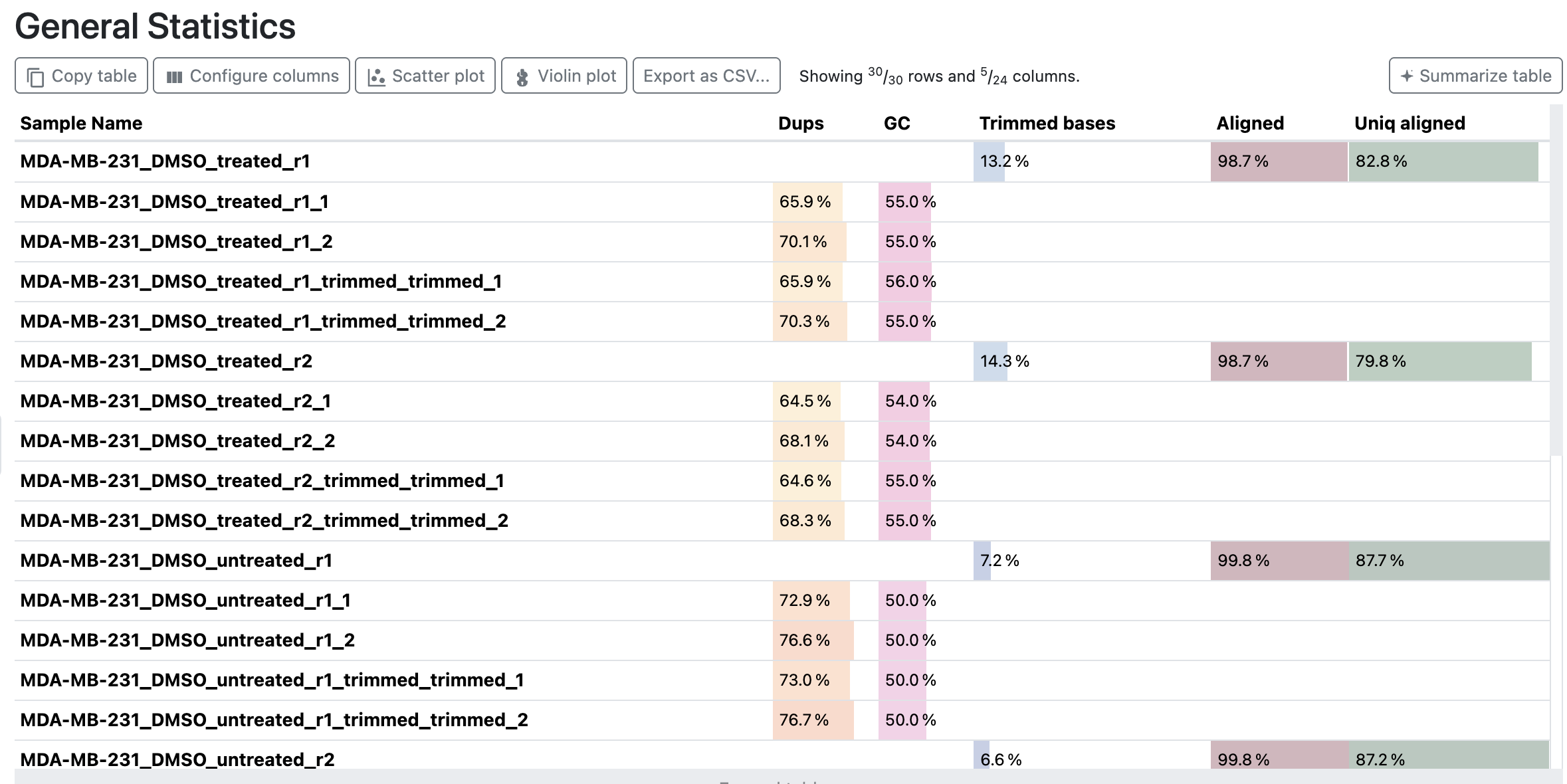
MultiQC aggregates results from all pipeline tools into a single report. Alongside the standard modules (FastQC read quality, Cutadapt trimming, Bowtie/Bowtie2/STAR alignment rates, and SAMtools flagstat/idxstats/stats), the pipeline adds custom summary tables that follow the samples through the RNA Framework steps. The screenshots below are from the human dataset (MDA-MB-231, DMS-MaP).
General Statistics
The standard MultiQC table, aggregating key per-sample metrics (read counts, duplication, GC, trimming, and alignment rate) across the QC modules:
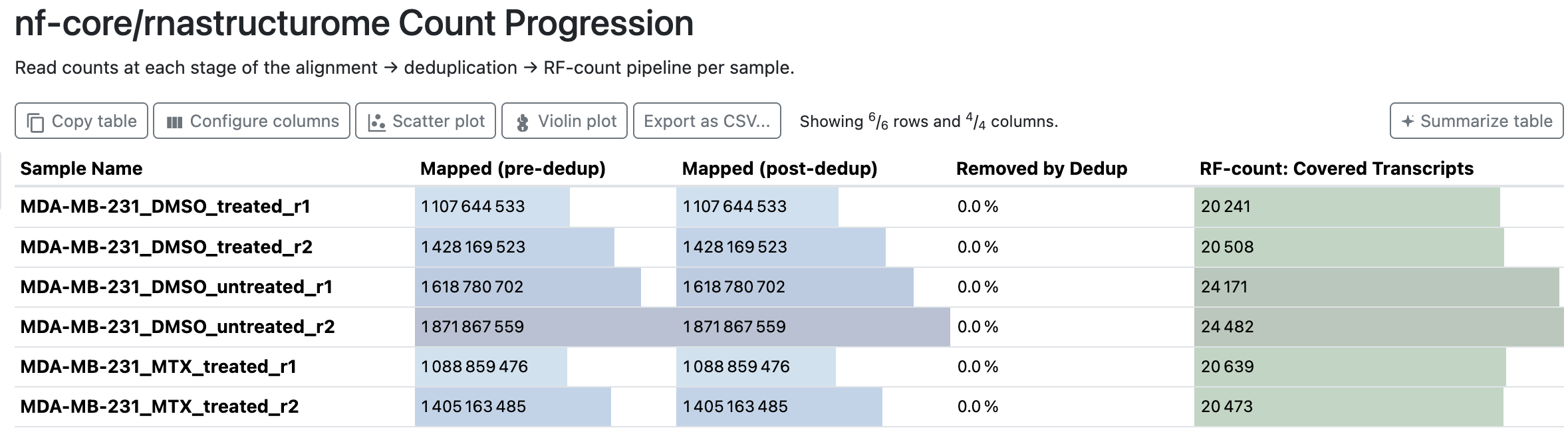
Count Progression
Per sample: reads mapped before and after deduplication, the fraction removed, and the number of transcripts rf-count covered. With the default --skip_markdup true (no UMIs) nothing is deduplicated, so “Removed by Dedup” is 0.0%.
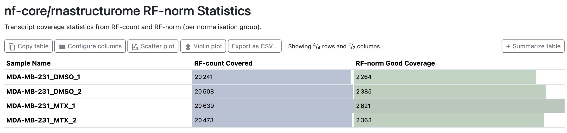
RF-norm Statistics
Per sample_group + replicate: how many of the covered transcripts pass rf-norm’s coverage filter (“Good Coverage”). The steep drop from ~20,000 covered transcripts to a few thousand well-covered ones is expected; only transcripts with enough per-base signal are worth normalising and folding.
RF-fold Statistics
Per sample_group: transcripts folded by rf-fold versus those discarded (too short, or without enough reactivity coverage to fold).

Replicate Correlation
Per sample_group: the replicate count and the mean pairwise Pearson and Spearman reactivity correlation, an at-a-glance reproducibility check. See rf-correlate for the per-replicate logs these are summarised from.

Pipeline information
Output files
pipeline_info/execution_report_<timestamp>.html: Nextflow execution report with per-process resource usage.execution_timeline_<timestamp>.html: Timeline view of task execution.execution_trace_<timestamp>.txt: Tab-separated trace file with runtime and resource metrics per task.pipeline_dag_<timestamp>.html: Directed acyclic graph of the pipeline.params_<timestamp>.json: Snapshot of all parameters used for the run.nf_core_rnastructurome_software_mqc_versions.yml: Software versions for all tools used.
Nextflow provides excellent functionality for generating various reports relevant to the running and execution of the pipeline. The files listed above are generated by default when the pipeline finishes. All files are timestamped so successive runs in the same output directory accumulate without overwriting prior results.